class: center, middle # Decision Tree CS534 - Machine Learning Yubin Park, PhD --- class: center, middle Suppose we have a dataset that has patients' medical notes and treatment records. We want to understand the relationship between patients' conditions and their treatments. --- class: center, middle So, how do doctors think? .figure-w500[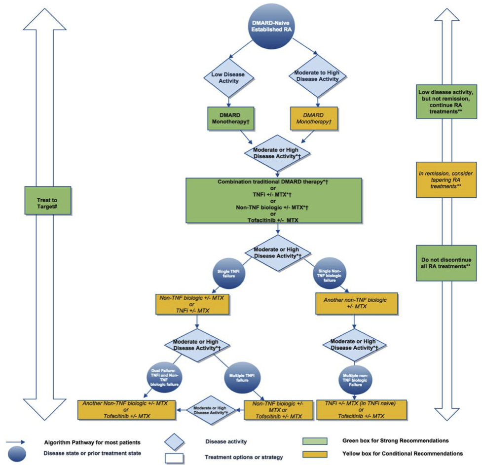] .reference[https://www.rheumatology.org/Portals/0/Files/ACR%202015%20RA%20Guideline.pdf] --- class: center, middle Just for fun... .reference[https://xkcd.com/1619/] .figure-w600[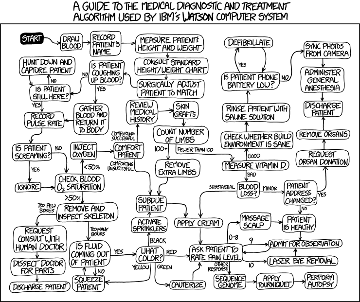] --- class: center, middle Such if-else rules may not be easily captured in linear models. **Enter Decision Tree.** --- class: center, middle Beside modeling such if-else rules, Decision Tree has many other advantages. .figure-350[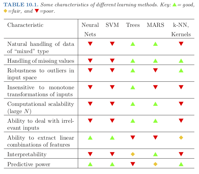] .reference[Chapter 10 of https://web.stanford.edu/~hastie/ElemStatLearn/] --- ## Decision Tree Decision Tree partitions data with if-else rules and assigns constant predictive values to those partitions. Mathematically, $$ f(\mathbf{x}) = \sum_{k} c_k I(\mathbf{x} \in R_k) $$ where `\(R_k\)` represents the `\(k\)`th partitioned region and `\(c_k\)` is the predictive value for the region. Finding the optimal partitions is NP-hard. Thus, we use a [greedy approach](https://en.wikipedia.org/wiki/Greedy_algorithm). e.g. partitioning data one by one. Decision Tree is also known as [Recursive Partitioning](https://en.wikipedia.org/wiki/Recursive_partitioning). --- class: center, middle Tree Representation .figure-300[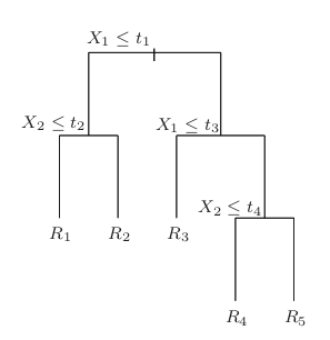] .reference[Chapter 9 of https://web.stanford.edu/~hastie/ElemStatLearn/] --- class: center, middle Partitioning Example .figure-300[] .reference[Chapter 9 of https://web.stanford.edu/~hastie/ElemStatLearn/] --- ## Decision Stump Decision Stump is a 1-level Decision Tree. Let's assume we have a **binary classification** dataset. We pick `\((x_{(j)}, v_s)\)` to split the dataset into two partitions. In other words, we have `\(\mathcal{D}_L = \{(\mathbf{x}, y) | x_{(j)} \leq v_s \}\)` (left node) and `\(\mathcal{D}_R = \{(\mathbf{x}, y) | x_{(j)} > v_s \}\)` (right node). For these partitions, define `\( q = \text{Average}(y | \mathcal{D}_L)\)` and `\( p = \text{Average}(y | \mathcal{D}_R)\)`. .center[.figure-200[]] --- ## Log-likelihood of Decision Stump Under this Decision Stump, we predict `\(p\)` if `\(x_{(j)} > v_s \)` and `\(q\)` if `\(x_{(j)} \leq v_s \)`. Let's assume `\(p > q\)` i.e. the right node will be the positive prediction node. We can draw a confusion table, and calculate the log-likelihood at each node. $$ \text{LL}_L = \text{FN} \times \log(q) + \text{TN} \times \log(1-q)$$ $$ \text{LL}_R = \text{TP} \times \log(p) + \text{FP} \times \log(1-p)$$ .pure-table.pure-table-bordered.pure-table-striped[ | | Left Node, `\(x_{(j)} \leq v_s\)` | Right Node, `\(x_{(j)} > v_s\)` | | ---- | --------------- | ------------------- | | Negative Class (`\(y=0\)`) | `\(\text{log-likelihood} = \text{TN} \times \log(1-q)\)` | `\(\text{FP} \times \log(1-p)\)` | | Positive Class (`\(y=1\)`) | `\(\text{FN} \times \log(q)\)` | `\(\text{TP} \times \log(p)\)` | ] --- ## Learning Decision Stump Pick a splitting variable and value pair, `\((x_{(j^*)}, v_{s^*})\)`, that gives the maximum log-likelihood. $$ (x\_{(j^\*)}, v\_{s^\*}) = \arg\max\_{(x\_{(j)}, v\_s)} \text{LL}\_L + \text{LL}\_R $$ We search all possible variable and value combinations, and select the best pair. This splitting criterion is called [Information Gain](https://en.wikipedia.org/wiki/Information_gain_in_decision_trees). $$ H(y | \text{Left}) = -q \log (q) - (1-q)\log(1-q) $$ $$ H(y | \text{Right}) = -p \log (p) - (1-p)\log(1-p) $$ $$\text{InfoGain} = - \text{size}_L H(y | \text{Left}) - \text{size}_R H(y | \text{Right}) $$ Note that maximum Information Gain is equivalent to maximum log-likelihood in this case. --- ## Stump to Tree To learn multi-level Decision Stump i.e. Decision Tree, we **recursively** iterate the same process on each partition. ```python def decision_tree(X, y, max_depth): n, m = X.shape if n < 3 or max_depth == 0: return np.mean(y) j_best, s_value = select_split_pair(X, y) left_idx = X[:,j_best] <= s_value right_idx = X[:,j_best] > s_value X_left, y_left = X[left_idx,:], y[left_idx] X_right, y_right = X[right_idx,:], y[right_idx] return {"split_var": j_best, "split_value": s_value, "left": decision_tree(X_left, y_left, max_depth-1), "right": decision_tree(X_right, y_right, max_depth-1)} ``` --- ## Other Splitting Criteria Information Gain is just one way of selecting the splitting variable and value. [CART (Classification and Regression Tree)](https://en.wikipedia.org/wiki/Predictive_analytics#Classification_and_regression_trees_.28CART.29) selects the splitting variable and value pair that mimizes [Gini Impurity](https://en.wikipedia.org/wiki/Decision_tree_learning#Gini_impurity) $$ \text{Gini}_L = 1 - q^2 $$ $$ \text{Gini}_R = 1 - p^2 $$ $$\text{Gini Impurity} = \text{size}_L \text{Gini}_L + \text{size}_R \text{Gini}_R $$ Various other splitting criteria exist in the form of: $$\min \text{size}_L h(q) + \text{size}_R h(p) $$ where `\(h(\cdot)\)` is a function that measures the impurity of the target variable, `\(y\)`. --- ## Regression Trees Decision Tree can be applied to regression tasks. To minimize Mean Squared Error, we find the best splitting pair that minimizes: $$ \text{size}_L \text{Var}(y | \text{Left}) + \text{size}_R \text{Var}(y | \text{Right}) $$ CART uses this splitting criterion for regression tasks. .center[.figure-200[]] .reference[Chapter 9 of https://web.stanford.edu/~hastie/ElemStatLearn/] --- ## Handling Missing Values Missing Values can be tricky to deal with when using machine learning algorithms. Many algorithms require either dropping samples with missing values or imputing missing values with some mechanisms. Decision Trees have a few additional options to deal with missing values: 1. For a categorical variable, we can treat "missing" as an additional categorical value. 1. For a numeric variable, we can send samples with missing values to the child node (left or right) that gives better prediction i.e. surrogate splits for missing values --- class: center, middle ## Limitations .figure-300[] .reference[Chapter 9 of https://web.stanford.edu/~hastie/ElemStatLearn/] --- class: center, middle ## Tree vs Linear Models .figure-300[] .reference[http://www.rnfc.org/courses/isl/Lesson%208/Videos/] --- class: middle, center Real-World Example .figure-350[] .reference[Chapter 9 of https://web.stanford.edu/~hastie/ElemStatLearn/] --- ## Bonsai-DT Numerous decision tree algorithms out there. - [C4.5](https://en.wikipedia.org/wiki/C4.5_algorithm) uses Information Gain to split nodes - [CART](https://en.wikipedia.org/wiki/Predictive_analytics#Classification_and_regression_trees_.28CART.29) uses Gini Impurity and Variance - [Hellinger Tree](https://www3.nd.edu/~nchawla/papers/DMKD11.pdf) uses Hellinger Distance - [Alph-Tree](https://ieeexplore.ieee.org/document/6399474) uses Alpha-Divergence You can make your decision tree by making a new splitting criterion (and that's it). This is my open-source project for easy-to-make custom decision trees. Check https://yubin-park.github.io/bonsai-dt/: .center[.figure-200[]] --- class: center, middle ## Questions?