class: center, middle # Evaluation Metrics & Strategies CS534 - Machine Learning Yubin Park, PhD --- class: center, middle We choose a loss function to fit a model. We choose an evaluation metric to evaluate the model. These two can be sometimes different. Loss Function `\(\neq\)` Evaluation Metric --- ## Evaluating Regression Tasks [Mean Squared Error (MSE)](https://en.wikipedia.org/wiki/Mean_squared_error) = `\( \frac{1}{n} \sum_{i=1}^{n} (y_i - \hat{y}_i)^2 \)` [Root Mean Sqaured Error (RMSE)](https://en.wikipedia.org/wiki/Root-mean-square_deviation) = `\(\sqrt{\text{MSE}}\)` [R-squared (or the coefficient of determination)](https://en.wikipedia.org/wiki/Coefficient_of_determination) = `\(1 - \frac{\text{MSE}}{\text{Var}(y)}\)` [Mean Absolute Error (MAE)](https://en.wikipedia.org/wiki/Mean_absolute_error) = `\(\frac{1}{n} \sum_{i=1}^{n} | y_i - \hat{y}_i |\)` [Mean Absolute Percentage Error (MAPE)](https://en.wikipedia.org/wiki/Mean_absolute_percentage_error) = `\(\frac{100}{n} \sum_{i=1}^{n} \frac{| y_i - \hat{y}_i |}{|y_i|}\)` [Median Absolute Error (MedAE)](https://scikit-learn.org/stable/modules/model_evaluation.html#median-absolute-error) = `\(\text{median}(|y_i - \hat{y}_i|)\)` [Mean Squared Logarithmic Error (MSLE)](https://scikit-learn.org/stable/modules/model_evaluation.html#mean-squared-logarithmic-error) = `\(\frac{1}{n} \sum_{i=1}^{n} (\log(1+y_i) - \log(1+\hat{y}_i))\)` --- ## Regression Evaluation Example ```python >>> from sklearn.metrics import mean_squared_error >>> y_true = [3, -0.5, 2, 7] >>> y_pred = [2.5, 0.0, 2, 8] >>> mean_squared_error(y_true, y_pred) 0.375 ``` .reference[https://scikit-learn.org/stable/modules/model_evaluation.html#mean-squared-error] ```python >>> from sklearn.metrics import mean_squared_log_error >>> y_true = [3, 5, 2.5, 7] >>> y_pred = [2.5, 5, 4, 8] >>> mean_squared_log_error(y_true, y_pred) 0.039... ``` .reference[https://scikit-learn.org/stable/modules/model_evaluation.html#mean-squared-logarithmic-error] --- ## Evaluating Classification Tasks [Confusion Matrix](https://en.wikipedia.org/wiki/Confusion_matrix) is the basis for evaluating classification algorithms. .pure-table.pure-table-bordered.pure-table-striped[ | | Predicted 0 (or Negative) | Predicted 1 (or Positive) | | ---- | --------------- | ------------------- | | Actual 0 (or Negative, N) | True Negative (TN) | False Positive (FP), Type I Error | | Actual 1 (or Positive, P) | False Negative (FN), Type II Error | True Positive (TP) | ] Accuracy = `\( \frac{TP + TN}{ P + N}\)` True Positive Rate (TPR) = `\( \frac{TP}{ TP + FN}\)` False Positive Rate (FPR) = `\( \frac{FP}{ FP + TN}\)` Positive Predictive Value (PPV, or Precision) = `\( \frac{TP}{TP + FP}\)` --- ## ROC Curve and Area Under the Curve (AUROC) .center[.figure-350[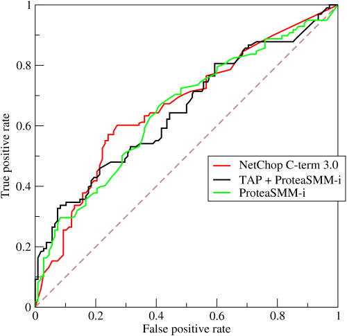]] .center[.reference[By BOR at the English language Wikipedia, CC BY-SA 3.0, https://commons.wikimedia.org/w/index.php?curid=10714489]] --- class: center, middle If a model is good, **in general**, AUROC should be above 0.5 and plausibly above 0.7-ish. Higher AUROCs, in general, imply better models. However, in practice, lower AUROC models may be preferred depending on the **shapes** of the ROC curves. --- ## Precision and Recall Precision = `\(\frac{TP}{TP + FP}\)` and Recall = `\(\frac{TP}{TP + FN}\)` .center[.figure-350[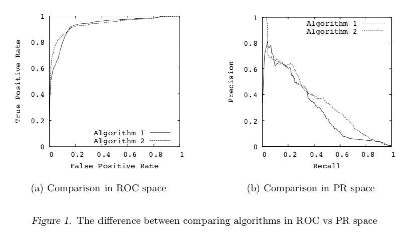]] .center[.reference[J. Davis and M. Goadrich, The Relationship Between Precision-Recall and ROC Curves. ICML 2006. https://www.biostat.wisc.edu/~page/rocpr.pdf]] --- ## Brier Score ROC and PR curves only care about the rankings of the predicted values. For example, if the target is `[0, 1]`, then predicted values of `[0.1, 0.9]` and `[0.4, 0.7]` would be the same in ROC and PR. On the other hand, [Brier Score](https://en.wikipedia.org/wiki/Brier_score) measures the accuracy of **probabilistic** predictions. For a binary classification problem where `\(y = \{0,1\}\)` and `\(\hat{y} \in [0, 1]\)`, $$\text{Brier Score (BS)} = \frac{1}{n}\sum_{i=1}^{n}(y_i-\hat{y}_i)^2$$ i.e. MSE applied to a binary classification task --- class: center, middle Now we know **what metrics** to measure. But, do we know **where/how** to apply? --- class: center, middle Why are we training a model? **To Predict Outcomes** (for the inputs you haven't seen yet) --- ## Train and Test By definition, you cannot measure the performance on the **unseen** data. However, you can simulate such performance assuming that the **unseen** data is not much different from the **data we already have**. Randomly split the data into two groups: - **Train set** for mimicking the data that we already have - **Test set** for mimicking the unseen data that we will have in the future .center[.figure-w650[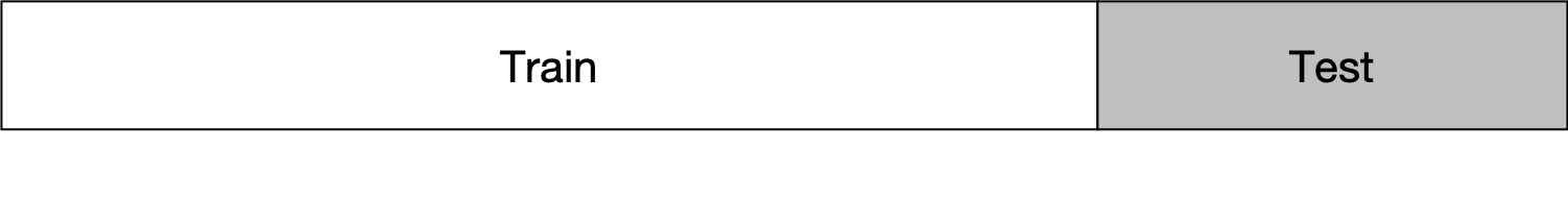]] Common split ratio: 70% for Train and 30% for Test You use the Test set only for measuring the evaluation metric. You **DO NOT** touch the Test set while training. --- ## K-Fold Cross-Validation One train/test split gives one estimate for the evaluation metric of interest. Can we trust the value? Can we get more estimates so that we can calculate variances of such estimates? Randomly split data into `\(k\)` partitions, and use one of the partition as a Test set, and then iterate over the other `\(k-1\)` Test sets. .center[.figure-250[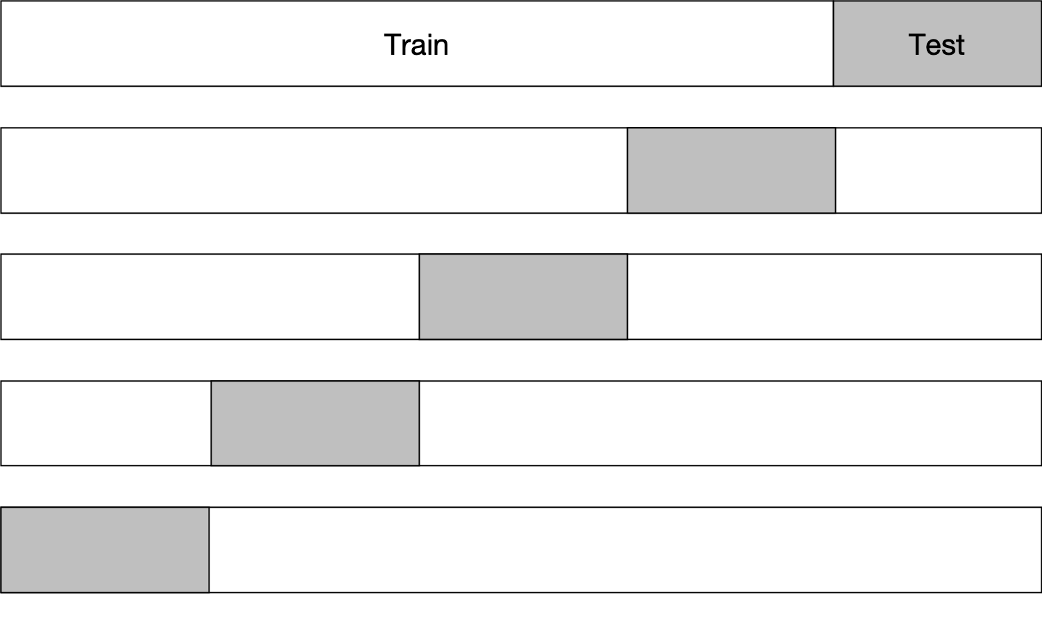]] --- ## Monte Carlo Cross-Validation The maximum number of estimates for K-Fold CV is K. For example, a 5-Fold CV will generate 5 evaluation metrics. Is 5 enough? .center[.figure-250[]] Doing a random sub-sampling multiple times. Test sets may have some overlapping data points between iterations. Can iterate as many as we want. --- class: center, middle Cross-validated performances should be **indicative** of real performance. We can choose the **best** model among our list of models based on the CV results. --- class: center, middle **A QUICK NOTE** A model has two types of parameters. Regular parameters (we just call "parameters"), and Hyperparameters, which we cannot estimate during training, such as `\(\lambda, \alpha\)` in Elastic-Net. If models have different hyperparameters, for now, let's just treat them **different** models. --- class: center, middle Example of Choosing the best `\(\lambda\)` in Elastic-Net .figure-350[] .reference[https://web.stanford.edu/~hastie/glmnet/glmnet_beta.html] --- class: middle ## Example of Bad Cross-Validation 1. Screen the predictors: find a subset of “good” predictors that show fairly strong (univariate) correlation with the class labels 2. Using just this subset of predictors, build a multivariate classifier. 3. Use cross-validation to estimate the unknown tuning parameters and to estimate the prediction error of the final model. What's wrong? .reference[Chapter 7 of https://web.stanford.edu/~hastie/ElemStatLearn/] --- class: middle ## Example of Correct Cross-Validation 1. Divide the samples into K cross-validation folds (groups) at random. 2. For each fold k = 1,2,...,K 2. For each fold k = 1,2,...,K 1. Find a subset of “good” predictors that show fairly strong (univariate) correlation with the class labels, using all of the samples except those in fold k. 2. Using just this subset of predictors, build a multivariate classifier, using all of the samples except those in fold k. 3. Use the classifier to predict the class labels for the samples in fold k. .reference[Chapter 7 of https://web.stanford.edu/~hastie/ElemStatLearn/] --- class: center, middle ## Questions?